Explanation
Explanation - Methodologies to Create the Layers
Radar Nowcasting for Pluvial Flood Hazard
Reflectivity observations from the pan-European EUMETNET OPERA composite are used to generate nowcasts of rainfall up to 5-hours ahead using the SBMCast model. The nowcasts are used to compute the pluvial flood hazard in urban areas layers, they are also one input to the computation of the River Flash Flood Impact layers.
Radar Observations
Reflectivity observations (units of dBZ) are obtained from the EUMETNET OPERA pan-European composite. Data are available every 15-minutes at a spatial resolution of 2-km. Reflectivity values are transformed into rainfall using a Z-R conversion.
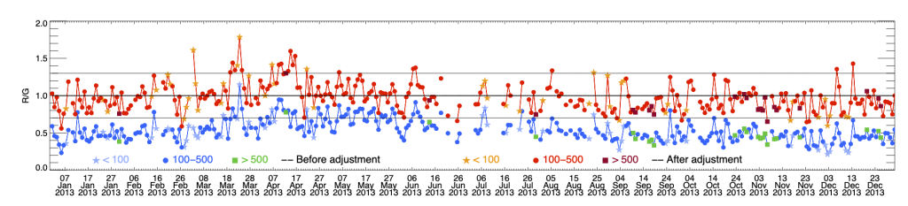
The converted rainfall values are bias corrected to ensure the values closely match those observed at gauging stations.The bias adjustment is done by multiplying the radar rainfall data by a correction factor, which is computed as the difference between the previous 30-days accumulated between the gauged value and the radar value. This computation is performed separately at each gauging station across a pan-European network, shown in the EFAS Raingauge accum. (24h) layer. The correction factors at all gauge station locations are then interpolated onto the same 2-km grid as the OPERA composite. This procedure to compute the correction factor is done once per day at 00 UTC. The gridded correction factor is multiplied to all radar rainfall values over the following 24-hour period to compute the bias corrected values. More details about the methodology can be found in Park et al., 2019.
Radar Rainfall Nowcasting
The bias corrected radar rainfall estimates are used to create a nowcast of rainfall up to 5-hours ahead with 15-minute time steps. The nowcast is created using the SBMCast model (Berenguer et al., 2011) which applies Lagrangian persistence to the previous 6-hours of bias corrected radar rainfall values. New nowcasts are made every 15-minutes when new radar observations become available.
Computation of Pluvial Hazard in Urban Areas
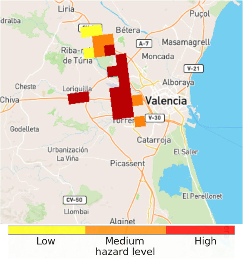
The pluvial flood hazard in urban areas layer is computed using the radar rainfall nowcasts computed in the previous step. The layer is only computed in urban areas, which are defined as 2-km grid cells in which ≥20% of the cell area is covered by urban or highly impermeable surfaces, defined from the CORINE land cover dataset. Within the 2-km grid cells identified as urban areas, the hourly rainfall accumulation in each 15-minute time step of the nowcast is compared against climatological thresholds associated with the 2-, 5- and 20-year return periods. These thresholds are computed from historical hourly rainfall accumulations from 8-years of bias corrected radar rainfall estimates. If the nowcasted rainfall in a given timestep and urban grid cell is expected to exceed one of the return period thresholds (Table 1), it is assigned to the corresponding hazard level.
| Return Period | Hazard Level |
|---|---|
| 2-year | Low |
| 5-year | Medium |
| 20-year | High |
| Table 1: Return period thresholds associated with each hazard level of the pluvial hazard in urban areas layer | |
References
- Berenguer, M., Sempere-Torres, D., Pegram, G.G.S. 2011. SBMcast – An ensemble nowcasting technique to assess the uncertainty in rainfall forecasts by Lagrangian extrapolation. Journal of Hydrology 404 (3-4), pp 226-240, 10.1016/j.jhydrol.2011.04.033
- Park, S., Berenguer, M., Sempere-Torres, D., & Von Lerber, A. 2024. The EUMETNET OPERA radar network: European-wide precipitation composites supporting rainfall-induced flash flood emergency management. In Responding to Extreme Weather Events (pp. 105–118). Wiley, https://doi.org/10.1002/9781119741374.ch5
Storm Impact Forecasting
The storm impact layers show lightning, wind and precipitation hazard and risk forecasted for the next three hours with 15-minute time steps. The products are shown in the same grid with the OPERA radar composites at spatial resolution of 2 kilometers.
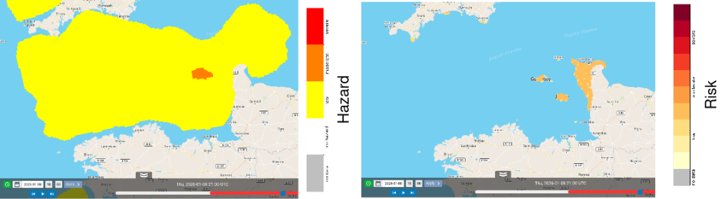
Storm hazard levels shown in the layers are divided into three classes having colours yellow (low), orange (moderate) and red (severe). The ranges of these classes are listed in Table 1. Precipitation below the minimum threshold of 1 mm/h or missing values are not shown.
| Lightning (flashes / 6*6 km / 30 minutes) | Precipitation (mm/h) | Wind (m/s) | |
| High | > 50 | > 10 | > 40 |
| Moderate | 10-50 | 5-10 | 30-40 |
| Low | 1-10 | 1-5 | 20-30 |
| No hazard | < 1 | < 1 | < 20 |
| Table 1: Ranges of hazard classes corresponding to the predicted meteorological quantities. | |||
The risk level is assigned based on exposure. In the storm risk products the exposure information is population density divided into classes listed in Table 2.
| Exposure | Population (people / km2) |
| High | > 50 |
| Moderate | 10-50 |
| Low | 1-10 |
| No exposure | < 1 |
| Table 2: Ranges for exposure classes based on population. | |
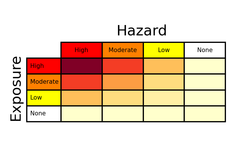
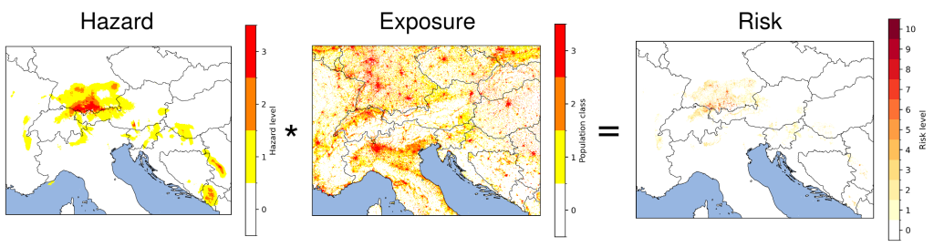
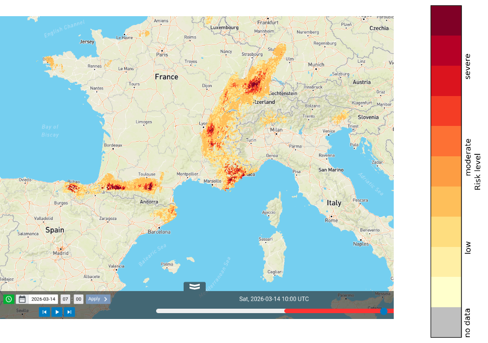
Storm risk is calculated from storm hazard by multiplying hazard level (0-3) with exposure level (0-3). This results into a risk level in the range between 0 (no risk) and 9 (severe) shown in yellow-to-red colours, as illustrated in Figures 1 and 2.
Precipitation hazard and risk
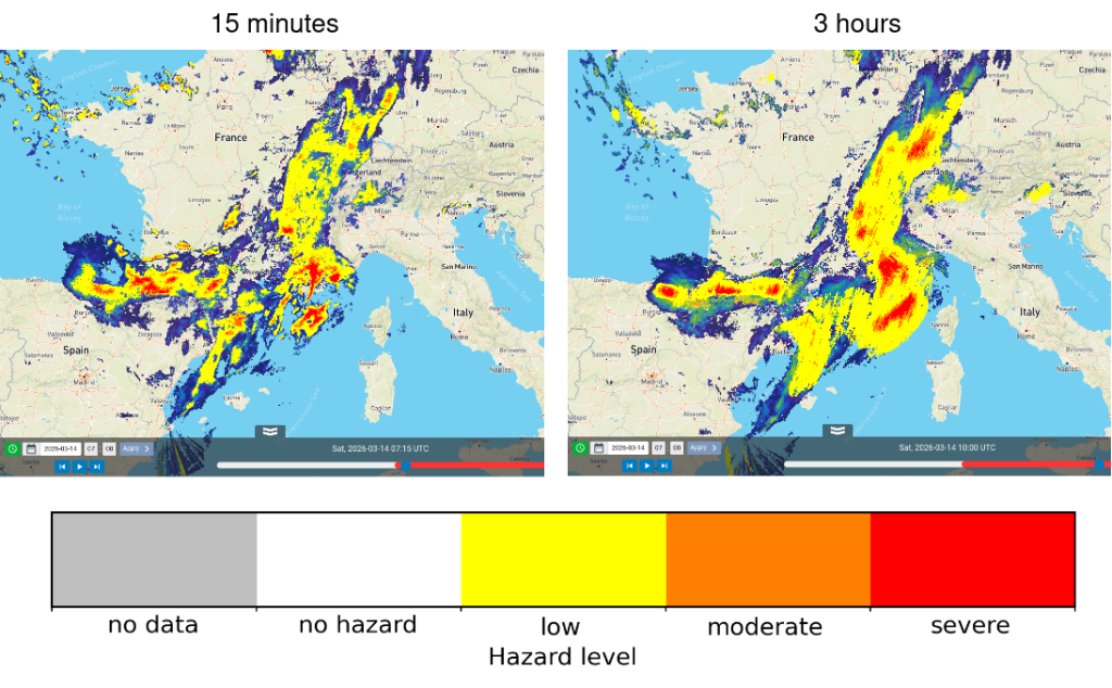
Nowcasts of precipitation hazard and risk are produced by using a convolutional neural network. The network architecture used here is Simpler yet Better Video Prediction (SimVP, Tan et al. 2025). Post-processing is applied to ensure that the predictions are consistent with the observed precipitation (Pulkkinen et al. 2019) and to generate ensemble nowcasts (Pulkkinen et al. 2021). Differently to the extrapolation method used in the meteorological layers group, the neural network is not only moving the precipitation but also predicting intensity changes. However, it generally cannot predict initiation of new storm cells. The neural network can also indicate uncertainty that increases with forecast length. This is illustrated in Figure 3 showing the changing intensity and smoothing to filter small-scale precipitation that cannot be predicted reliably. The corresponding risk nowcast is shown in Figure 4.
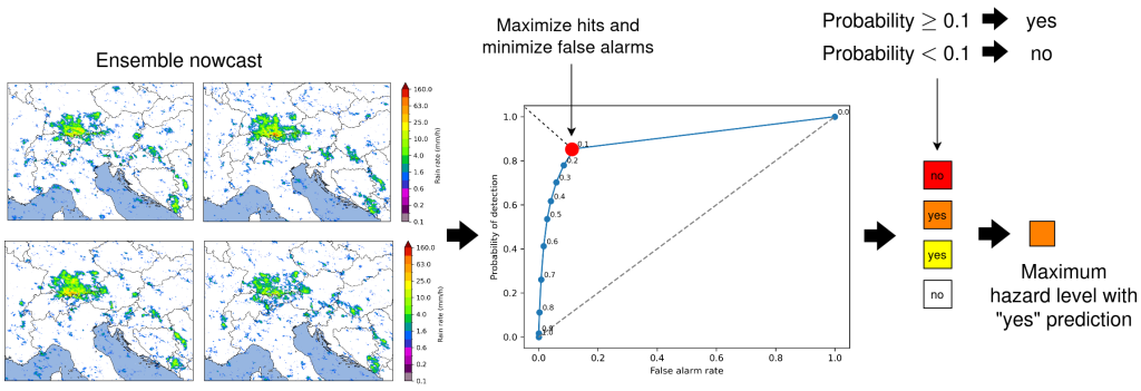
The precipitation hazard levels are estimated from an ensemble of nowcasts representing alternative scenarios. For each hazard level displayed in Table 1, the exceedance probability of each level in each grid cell is estimated from the ensemble. The probabilities are converted into a “yes” or “no” prediction for the exceedance. The conversion is done by using probability thresholds that minimize false alarms and maximize hits. Then a maximum hazard level with a “yes” prediction is taken. This is illustrated in Figure 5. However, the probability information is not currently shown to the user. This will be implemented in a future version.
Lightning hazard and risk
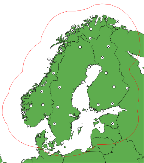
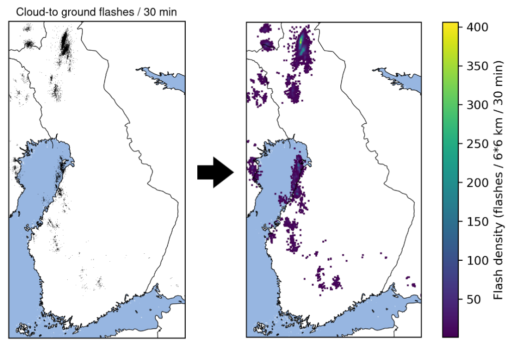
Lightning hazard and risk products are implemented in a limited area. Cloud-to-ground flash observations are used from the NORDLIS observation network shown in Figure 6. The observations are gridded into flash density, as illustrated in Figure 7. Each grid cell in the flash density contains the number of flashes in a 6 x 6 km spatial window centered at the cell and in a time window containing the previous 30 minutes. Nowcasts of the flash density are produced by using the extrapolation method implemented in pySTEPS (Pulkkinen et al. 2019) without predicting intensity changes. Then the method described above is applied to assign hazard and risk levels. This is done from the deterministic nowcast without generating an ensemble. Due to limitations of the extrapolation method, it is advised to use this product only when looking at the next 30 minutes. Predicting intensification or weakening of lightning activity will be implemented in a future version.
Wind hazard and risk
The wind hazard and risk products are based on wind u- and v-components from ECMWF’s Integrated Forecasting System (IFS) model. Deterministic HRES forecasts at height of 10 meters above ground level are used. The forecasts are queried from the ECMWF data feed via the API provided by the FMI. In this way new forecasts are available every 12 hours with 3-hour time steps. The u- and v-components are processed into wind speed (m/s). Interpolation is applied to estimate the wind speed at 15-minute time steps shown on the platform in the 2 x 2 km OPERA grid (the original grid is in latitude-longitude projection with resolution of 0.1o). The resulting hazard and risk products by applying the above method are illustrated in Figure 8.
References
- Pulkkinen S., Chandrasekar, V., and Niemi, T., 2021, Lagrangian Integro-Difference Equation Model for Precipitation Nowcasting, J. Atmos. Ocean. Technol., 38, 2125-2145, https://doi.org/10.1175/JTECH-D-21-0013.1
- Pulkkinen, S., Nerini, D., Pérez Hortal A. A., Velasco-Forero, C., Seed, A., Germann, U. and Foresti, L., 2019, Pysteps: an open-source Python library for probabilistic precipitation nowcasting (v1.0), Geosci. Model Dev., 12, 4185-4219, https://doi.org/10.5194/gmd-12-4185-2019
- Tan, C., Gao, Z., Li, S. and Li, S. Z., 2025, SimVPv2: Towards Simple Yet Powerful Spatiotemporal Predictive Learning, IEEE Trans. Multimedia, 27, 5170 – 5184, https://doi.org/10.1109/TMM.2025.3543051
River Flash Flood Impact Forecasting
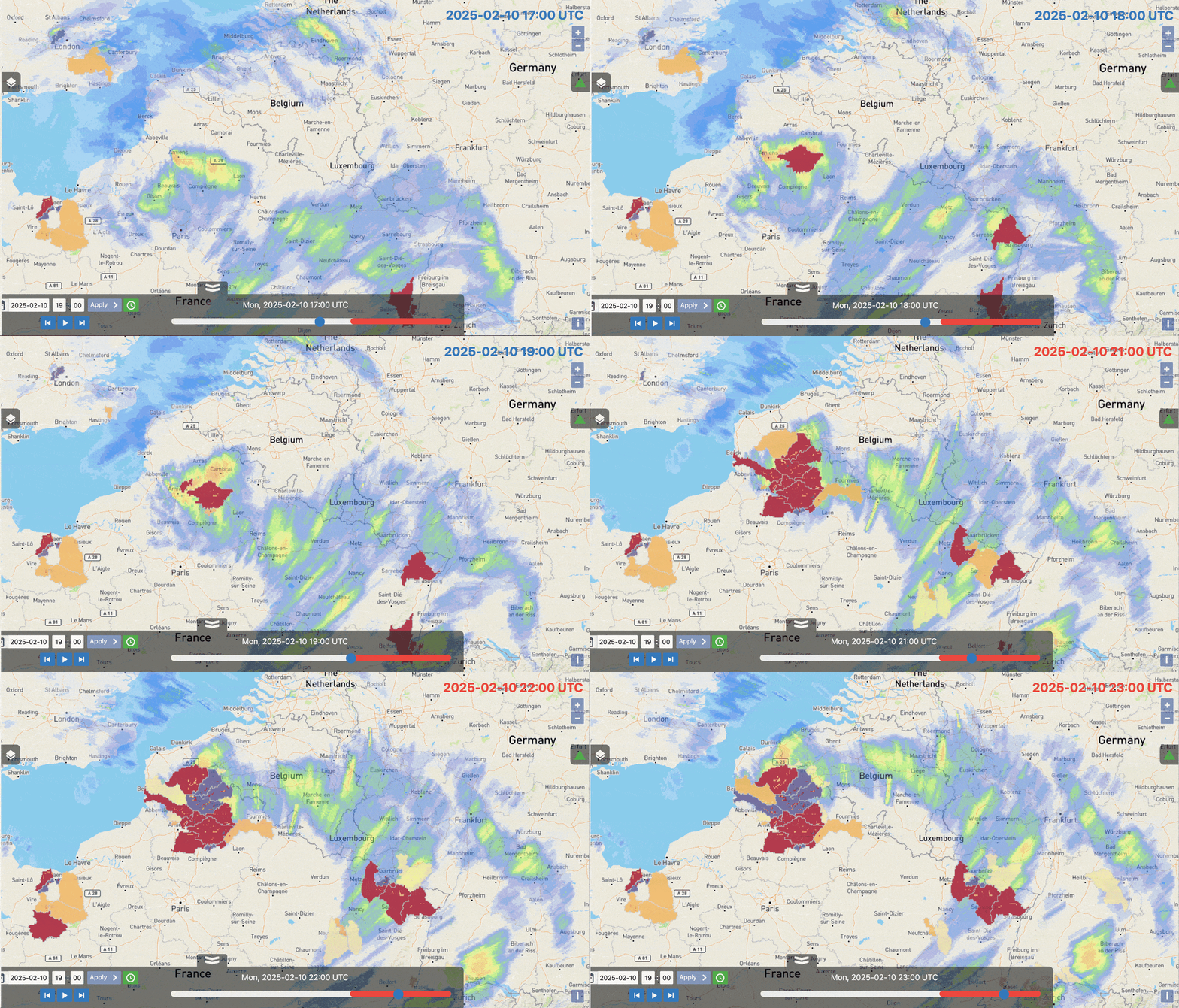
The river flash flood impact product identifies rivers, with an upstream drainage area greater than 50 km2 and less than 2000 km2, where there is a risk of flash flood impacts over the next 5-days. An animated example of this product is shown below in Figure 1.
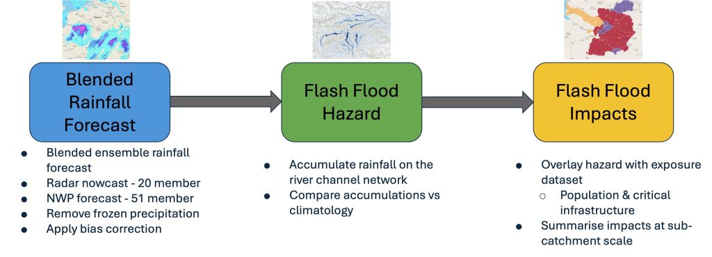
The product is created in three steps (Figure 2):
- Creating a blended ensemble precipitation forecast by combining radar nowcasts and ECMWF IFS NWP.
- Calculating the flash flood hazard in the river network, expressed as the probability of exceeding the 2-year return period threshold.
- Converting the forecasted flash flood hazard into potential impacts by combining with a combined exposure layer (which accounts for population and critical infrastructure).
Blended Ensemble Precipitation Forecasting
For the first 5-hours lead time, an hourly ensemble forecast is created by blending the radar nowcast and the ECMWF IFS. Beyond 5-hours lead time, the precipitation forecast is obtained only from the ECMWF IFS ensemble at 6-hourly timesteps up to 120-hours lead time. The 80th percentile from the ensemble forecast is computed and used to create the Seamless Precipitation Accumulation and Hourly precipitation 80th percentile products.
Blended Precipitation for Lead Times 0-5 hours
For the first 5-hours of the forecast lead time, the precipitation accumulations have been obtained by the blending of the:
- 20-member ensemble nowcast of 1-hour accumulated precipitation, generated using SBMcast (Berenguer et al., 2011) using the gauge-adjusted rainfall estimates from the pan-European OPERA radar composite (Park et al. 2019). These have a spatial resolution of 2 km.
- 51-member ensemble forecast of 1-hour accumulated precipitation generated by Numerical Weather Prediction (NWP) from the ECMWF Ensemble Prediction System (EPS). These data have a spatial resolution of 9 km, they are interpolated onto the same 2 km resolution as the nowcast data using a nearest neighbour method.
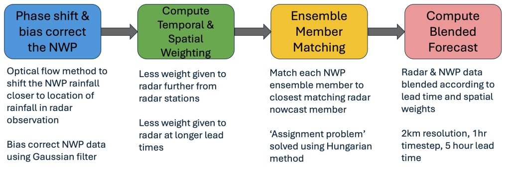
The blending technique (Wong et al. 2009) is applied for the first 5-hours and involves 4 steps (Figure 3):
-
Phase shifting and bias correcting the NWP forecasted precipitation to ensure a closer between the locations of rain in the NWP and radar nowcasts
- For each member of the NWP forecast, an optical flow method is used to compute the phase shift in the first 1-hour time step between the forecasted precipitation in the NWP ensemble member and the first ensemble member of the nowcast
- The computed phase shift is applied to the accumulated precipitation forecasted by the NWP for each hourly time step up to a lead time of 6 hours
- For each member of the NWP forecast, a scale factor is computed in the first 1-hour time step in each grid cell between the accumulated precipitation from the first member of the ensemble nowcast and the NWP forecast and the first member of the ensemble nowcast at the first time step is computed
- A Gaussian filter is applied to the scale factor grid which was computed above
- The phase shift corrected accumulated precipitation forecasted by the NWP in each time step, up to a maximum lead time of 6 hours, is multiplied by the scale factor
-
A spatial weighting factor, ws, is computed by applying a hyperbolic tangent function to the area within the EUMETNET OPERA radar coverage, to give greater weight to the radar nowcast data in areas which are closer to the locations of radar stations
- A temporal weighting factor, wt, is computed for each 1-hour time step of the 6-hour forecast lead time using a hyperbolic tangent function. This gives more weight to the accumulated precipitation from the NWP forecast at longer lead times
- Ensemble member matching of each member of the phase shifted and bias corrected NWP ensemble forecast (see the first two steps) to the member of the radar-based nowcast which has the smallest difference – computed as the sum of the square differences divided by the sum of the normalised square differences
- Compute blended forecast, TpBlend, by adding each ensemble member, m, of the phase shifted and bias corrected NWP precipitation forecast, TpNWP, to the precipitation from the closest matching member of the radar-based nowcast, TpNowcast. Spatial and temporal weighting factors (ws and wt respectively) are multiplied to both the NWP and nowcast precipitation forecasts. This produces a blended forecast of accumulated precipitation at each 1-hour time step, t, for the first 6 hours lead time:
NWP Precipitation for Lead Times 6-120 hours
For lead times from 6-120 hours, the accumulated precipitation is only from the 51-members ECMWF ensemble NWP forecast. This dataset has a spatial resolution of 9 km, it is regridded onto the same 2 km grid as the radar-based nowcasts using a nearest neighbour method. The forecasts at this lead time range have a time step of 6-hours.
Calculating the 80th Percentile
At each 1-hour time step for the first 5-hours lead time, the accumulated precipitation associated with the 80th percentile is computed from the 51-member blended forecast and is displayed in the Hourly Precipitation 80th percentile layer. For each 6-hour time step for lead times from 6 to 120-hours, the accumulated precipitation associated with the 80th percentile is computed from the 51-member ECMWF NWP forecasts. The total precipitation associated with the 80th percentile is accumulated over lead time windows of 0-6, 6-24, 24-48 and 48-120 hours and is displayed in the Seamless Precipitation Accumulation layer.
Computation of Flash Flood Impacts on the River Network
Flash flood impacts on the river network are computed in two steps: 1) a river flash flood hazard is computed by accumulating rainfall on the river network and computing the exceedance probability of the 2-year return period, 2) the exceedance probability is then overlaid with exposure information to estimate the flash flood impact level.
River Flash Flood Hazard Forecasts
Flash flood hazard is computed in three steps (Figure 4): 1) rainfall is accumulated on a channel network, 2) the accumulated rainfall is compared against the 2-year return period climatological threshold to identify grid cells where it is exceeded, 3) the 2-year return period exceedance is computed for all forecast ensemble members to compute the probability of exceedance.
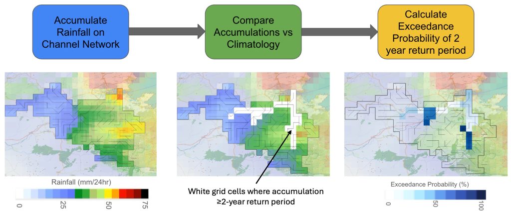
At each time step of the forecast, at each grid cell with an upstream drainage area ≥50 km2 and ≤2000 km2, the rainfall is summarised as the total amount which was forecasted to fall across the area upstream of the grid cell over the preceding time period equal to the river’s time of concentration, Tc. The time of concentration refers to the time between rain falling and the river reaching its peak, it was computed at each grid cell using the method of Giandotti, 1934 which was derived for small rural catchments:
where A = upstream drainage area (km2), L = the slope length (km) and H = difference between the mean elevation in the area upstream of the grid cell and the elevation of the grid cell (m)
- 8-year gauge-adjusted OPERA radar rainfall data
- A dataset of 20-year reforecasts obtained with ECMWF Integrated Forecasting System (IFS)
At each location on the river network and each forecast time step, the total number of ensemble members which exceed the summarised rainfall associated with the 2-year return period is computed and then divided by the total number of ensemble members (51) to give a probability of exceedance (%).
River Flash Flood Impact Prediction
River flash flood impact level is computed by intersecting the flash flood hazard, computed in the previous step, with a static dataset of combined population and critical infrastructure exposure (Figure 5).
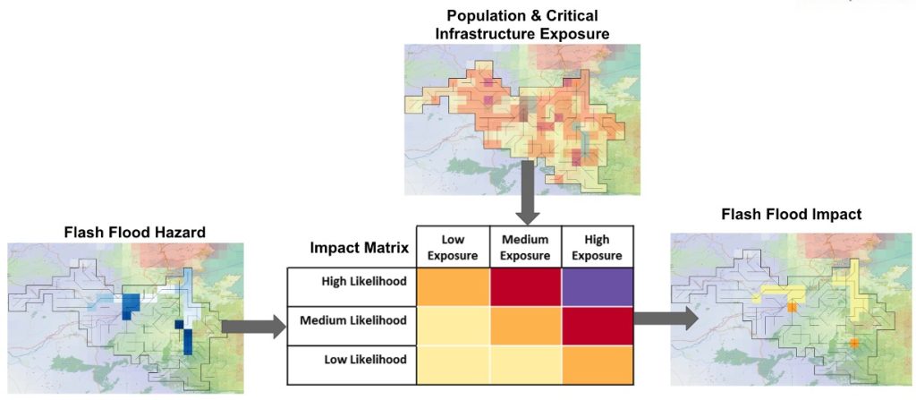
The exposure data accounts for population and critical infrastructure in the form of health, education, transport, and energy generation facilities. Population data were obtained from the GHSL (Global Human Settlement Layer), the critical infrastructure data were from HARCI-EU within EU member states and OpenStreetMap for non-EU member states. Data for each of these five categories was harmonised and combined with equal weighting to create a combined exposure layer whose values ranged from 1.0-2.0. The resulting dataset is available on the web platform as the Exposure layer.
The river flash flood impact level is computed at each time step by intersecting the river flash flood hazard forecast with the combined exposure dataset. The low, medium, and high values for flash flood hazard likelihood on the y-axis of the impact matrix indicate where there is a 5%-50%, 50%-80%, and >80% probability of exceeding the 2-year return period threshold.
The categories for low, medium, and high exposure, on the x-axis of the impact matrix, relate to combined exposure values of 1.0-1.3, 1.3-1.6 and 1.6-2.0 respectively. These categories were chosen based on the statistical distribution of exposure values across the EFAS domain, and consequently 81.0% of the exposure values are classified as low exposure, 8.0% as medium exposure and 1.2% as high exposure. This reflects the reality that most grid points in Europe have a low population density and with few exposed critical infrastructures
This combination of flash flood hazard level with exposure gives impact levels for each grid cell on the river network at each time step of the 120 hour forecast period. The data for the first 5-hours lead time are visualised on the web platform as the River flash flood impact over river network layer.
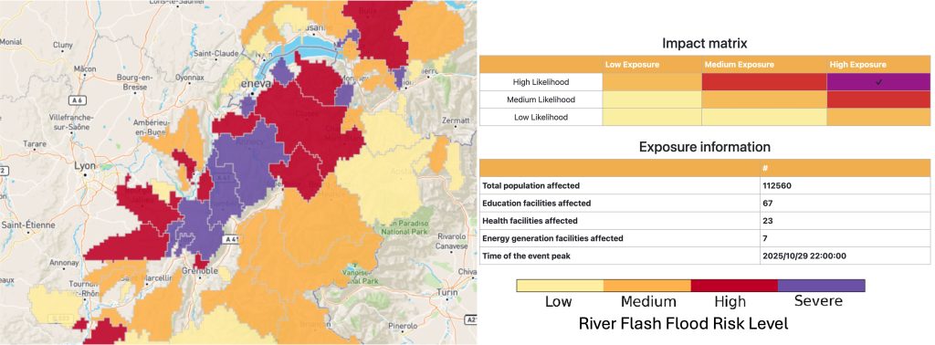
The forecasted river flash flood impact level is summarised onto river sub-catchments by computing the 90th percentile of the flash flood impact level across all grid cells within each sub-catchment. The 90th percentile was chosen rather than the maximum to prevent sub-catchments being assigned an impact level based upon a single grid cell value. The sub-catchment summary is displayed on the web platform as the River flash flood impact over sub-catchment layer.
Flash flood impacts in each sub-catchment are also summarised over lead time windows of 0-6, 6-24, 24-48 and 48-120 hours, by computing the maximum flash flood impact level in each grid cell in each lead time window. Then the 90th percentile of the flash flood impact level for each lead time window is computed in each sub-catchment. The results are shown in the Flash flood impact over sub-catchment layer (Figure 6). When this layer is clicked in the web platform, a pop out window appears containing additional information about the total affected population and the critical infrastructure assets. These are computed by summarising the total population and infrastructure assets in grid cells where the forecasted flash flood impact level is low or above. The time of the peak is computed by identifying the lead time when the maximum impact level is forecasted.
References
- Berenguer, M., Sempere-Torres, D. and Pegram, G, 2011: SBMcast – An ensemble nowcasting technique to assess the uncertainty in rainfall forecasts by Lagrangian extrapolation. Journal of Hydrology, 404(3), 226-240
- Park, S., Berenguer, M. and Sempere-Torres, D, 2019: Long-term analysis of gauge-adjusted radar rainfall accumulations at European Scale. Journal of Hydrology, 573, 768-777
- Wong, W., Yeung, L., Wang, Y. and Chen, M, 2009: Towards the Blending of NWP with Nowcast – Operation Experience in B08FDP. WMO Symposium on Nowcasting, 30 Aug- 4 Sep, Whistler, Canada.